Smooth a signal

%matplotlib inline
import numpy as np
from matplotlib import pyplot as plt
import rampy as rp

# the following code is for the rendering of plotly graphs in Rampy docs, you don't need it
# Set renderer for Jupyter notebooks
import plotly.io as pio
pio.renderers.default = 'notebook'

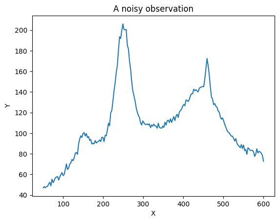
First we creating a fake, noisy signal

nb_points  = 200
x = np.linspace(50, 600, nb_points)

# gaussian peaks
p1 = 20.0 * np.exp(-np.log(2) * ((x-150.0)/15.0)**2)
p2 = 100.0 * np.exp(-np.log(2) * ((x-250.0)/20.0)**2)
p3 = 50.0 * np.exp(-np.log(2) * ((x-450.0)/50.0)**2)
p4 = 20.0 * np.exp(-np.log(2) * ((x-350.0)/300)**2)
p5 = 30.0 * np.exp(-np.log(2) * ((x-460.0)/5.0)**2)

# background: a large gaussian + linear
bkg = 60.0 * np.exp(-np.log(2) * ((x-250.0)/200.0)**2) + 0.1*x

#noise
noise = 2.0 * np.random.normal(size=nb_points)

#observation
y = p1 + p2 + p3 + p4 + p5 + noise +bkg


plt.plot(x, y)
plt.xlabel('X')
plt.ylabel('Y')
plt.title('A noisy observation')

Text(0.5, 1.0, 'A noisy observation')

To smooth this signal, we can use the rampy.smooth function. It has 10 different smnoothings algorithms.

Spline, Savitsky-Golay and Whittaker smoothing are available as: - GCVSmoothedNSpline (Generalised Cross Validated Spline, see scipy.interpolate.make_smoothing_spline doc) - DOFSmoothedNSpline (Degree of Freedom spline, see gcvspline doc) - MSESmoothedNSpline (Mean Square Error spline, see gcvspline doc) - savgol, the scipy Savitsky-Golay filter - whittaker, a Whittaker smoother (see rampy.whittaker())

Moving window smoothings are available by setting the method to: - flat, a flat window smoothing - hanning, a hanning window smoothing - hamming, a hamming window smoothing - bartlett, a bartlett window smoothing - blackman, a blackman window smoothing

See the smooth function help for more details on parameters

y_smo_1 = rp.smooth(x,y,method="GCVSmoothedNSpline")
#y_smo_2 = rp.smooth(x,y,method="DOFSmoothedNSpline") # activate only if you have gcvspline install (see charlesll/gcvspline on Github)
#y_smo_3 = rp.smooth(x,y,method="MSESmoothedNSpline") # activate only if you have gcvspline install (see charlesll/gcvspline on Github)
y_smo_4 = rp.smooth(x,y,method="savgol",window_length=5,polyorder=2)
y_smo_5 = rp.smooth(x,y,method="whittaker",Lambda=10**0.5)
y_smo_6 = rp.smooth(x,y,method="flat",window_length=5)
y_smo_7 = rp.smooth(x,y,method="hanning",window_length=5)
y_smo_8 = rp.smooth(x,y,method="hamming",window_length=5)
y_smo_9 = rp.smooth(x,y,method="bartlett",window_length=5)
y_smo_10 = rp.smooth(x,y,method="blackman",window_length=5)

Figures

To do a figure that allows interactively comparing the smoothing results, we use the rampy.plot_spectrum function:

fig = rp.plot_spectrum(x, y,
                       smoothed_signals=[y_smo_1, y_smo_4, y_smo_5, y_smo_6, y_smo_7, y_smo_8, y_smo_9, y_smo_10],
                       smoothed_labels=["GCVSmoothedNSpline", "savgol", "whittaker", "flat", "hanning", "hamming", "bartlett", "blackman"])
fig.show()

We can compare in more details the Sav-Gol, GCV spline and Whittaker method:

fig = rp.plot_spectrum(x, y, smoothed_signals=[y_smo_1, y_smo_4, y_smo_5],
                          smoothed_labels=["GCV spline", "Sav Gol", "Whittaker"])
fig.show()