Baseline
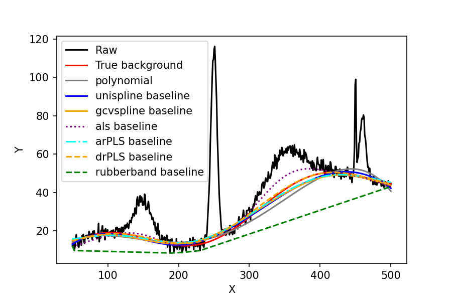
Rampy allows you to fit polynomial, spline, generalized cross-validated spline, logarithms, exponential, ALS, arPLS, drPLS, rubberband and whittaker baselines to your spectra, in order to remove the background.
Below you will find the documentation of the relevant functions, and have a look at the example notebooks too: Example notebooks
- rampy.baseline(x_input: ndarray, y_input: ndarray, method: str = 'poly', **kwargs) tuple
Subtracts a baseline from an x-y spectrum using various methods.
This function performs baseline subtraction on spectroscopic data by fitting a model to the background signal. It supports multiple correction methods, including polynomial fitting, splines, and advanced penalized least squares techniques.
- Parameters:
x_input (ndarray) – The x-axis values (e.g., wavelength or wavenumber).
y_input (ndarray) – The y-axis values (e.g., intensity or absorbance).
method (str, optional) –
The method used for baseline fitting. Default is “poly”. Available options:
”poly”: Polynomial fitting. Requires polynomial_order.
”unispline”: Spline fitting using Scipy’s UnivariateSpline. Requires s.
”gcvspline”: Spline fitting using GCVSpline. Requires s and optionally ese_y.
”gaussian”: Gaussian function fitting. Requires p0_gaussian.
”exp”: Exponential background fitting. Requires p0_exp.
”log”: Logarithmic background fitting. Requires p0_log.
”rubberband”: Rubberband correction using convex hull interpolation.
”als”: Asymmetric Least Squares correction. Requires lam, p, and niter.
”arPLS”: Asymmetrically Reweighted Penalized Least Squares smoothing. Requires lam and ratio.
”drPLS”: Doubly Reweighted Penalized Least Squares smoothing. Requires niter, lam, eta, and ratio.
”whittaker”: Whittaker smoothing with weights applied to regions of interest. Requires lam.
”GP”: Gaussian process method using a rational quadratic kernel.
**kwargs –
Additional parameters specific to the chosen method. - roi (ndarray): Regions of interest for baseline fitting. Default is the entire range of x_input. - polynomial_order (int): Degree of the polynomial for the “poly” method. Default is 1. - s (float): Spline smoothing coefficient for “unispline” and “gcvspline”. Default is 2.0. - ese_y (ndarray): Errors associated with y_input for the “gcvspline” method.
Defaults to sqrt(abs(y_input)) if not provided.
lam (float): Smoothness parameter for methods like “als”, “arPLS”, and others. Default is 1e5.
p (float): Weighting parameter for ALS method. Recommended values are between 0.001 and 0.1. Default is 0.01.
ratio (float): Convergence ratio parameter for arPLS/drPLS methods. Default is 0.01 for arPLS and 0.001 for drPLS.
niter (int): Number of iterations for ALS/drPLS methods. Defaults are 10 for ALS and 100 for drPLS.
eta (float): Roughness parameter for drPLS method, between 0 and 1. Default is 0.5.
p0_gaussian (list): Initial parameters [a, b, c] for Gaussian fitting: (y = a cdot exp(-log(2) cdot ((x-b)/c)^2)). Default is [1., 1., 1.].
p0_exp (list): Initial parameters [a, b, c] for exponential fitting: (y = a cdot exp(b cdot (x-c))). Default is [1., 1., 0.].
p0_log (list): Initial parameters [a, b, c, d] for logarithmic fitting: (y = a cdot log(-b cdot (x-c)) - d cdot x^2). Default is [1., 1., 1., 1.].
- Returns:
corrected_signal (ndarray): The signal after baseline subtraction. baseline_fitted (ndarray): The fitted baseline.
- Return type:
tuple
- Raises:
ValueError – If the specified method is not recognized or invalid parameters are provided.
Notes
The input data is standardized before fitting to improve numerical stability during optimization. The fitted baseline is transformed back to the original scale before subtraction.
Examples
Example with polynomial baseline correction:
>>> import numpy as np
>>> x = np.linspace(50, 500, nb_points)
>>> noise = 2.0 * np.random.normal(size=nb_points)
>>> background = 5 * np.sin(x / 50) + 0.1 * x
>>> peak = rampy.gaussian(x, 100.0, 250.0, 7.0)
>>> y = peak + background + noise
>>> roi = np.array([[0, 200], [300, 500]])
>>> corrected_signal, baseline = baseline(x, y, method="poly", roi = roi, polynomial_order=5)
Example with GCVSpline algorithm:
>>> corrected_signal, baseline = baseline(x, y, method="gcvspline", roi=roi, s=2.0)
Example with Whittaker smoothing:
>>> corrected_signal, baseline = baseline(x, y, method="whittaker", roi=roi)
Example with Gaussian process:
>>> corrected_signal, baseline = baseline(x, y, method="GP", roi=roi)
Example with rubberband correction:
>>> corrected_signal, baseline = baseline(x, y, method="rubberband")
Example with ALS algorithm:
>>> corrected_signal, baseline = baseline(x, y, method="als", lam=1e5, p=0.01)
For some baseline types, individual baseline functions also can be used, if you are interested:
- rampy.rubberband_baseline(x: ndarray, y: ndarray) ndarray
Perform rubberband baseline correction.
- Parameters:
x (ndarray) – The x-axis values.
y (ndarray) – The y values corresponding to x.
- Returns:
baseline_fitted – The fitted baseline.
- Return type:
ndarray
- Raises:
ValueError – If the convex hull does not have enough points for interpolation.
- rampy.als_baseline(y: ndarray, lam: float, p: float, niter: int) ndarray
Asymmetric Least Squares baseline fitting.
- rampy.arPLS_baseline(y: ndarray, lam: float, ratio: float) ndarray
Asymmetrically Reweighted Penalized Least Squares baseline fitting.
- rampy.drPLS_baseline(y: ndarray, niter: int, lam: float, eta: float, ratio: float) ndarray
Doubly Reweighted Penalized Least Squares baseline fitting.